[JV]
Part 1: scalars to tensors, backprop by hand
Built a reverse-mode autodiff engine from scratch: a scalar Value engine, an MLP trained on top of it, then a NumPy-backed Tensor class with broadcasting, batched matmul, and softmax.
- Backprop is the chain rule applied to a graph. Traversal order and gradient accumulation (
+=, not=) are the only non-obvious parts - Broadcasting on the forward pass must be explicitly undone (summed) on the backward pass
- Composing correct primitives is a debugging strategy: ops built from verified pieces inherit their correctness
- A failing test is not proof the math is wrong. Check precision mismatches (
float32vsfloat64) first
Building a character-level transformer on top of this engine: self-attention, layer norm, feedforward block, cross-entropy loss, and Adam. Attention is free (just matmul + softmax); the missing pieces are embedding-lookup indexing, layer norm, and a log primitive for cross-entropy.
This project implements a reverse-mode automatic differentiation engine from scratch in Python and NumPy to understand the mechanics behind gradient computation.
It covers a scalar engine, an MLP trained on top of it, and a generalization to NumPy-backed tensors. PyTorch is used only as a reference in the test suite: every gradient the engine computes is checked against what PyTorch produces for the same expression.
The resulting engine serves as the foundation for implementing a transformer from first principles.
The idea underneath .backward()
Any arithmetic expression can be represented as a graph:
This builds a directed acyclic graph. a and b feed into a multiply node, that combines with c at an add node, and the result goes through tanh to produce L. Training means computing for every parameter : how much does changing this weight change the loss.
There are two ways to get every one of those partial derivatives:
- Forward-mode, where you propagate a derivative forward through the graph one input at a time. The cost scales with the number of inputs.
- Reverse-mode, where you propagate a derivative backward from the output, once. The cost scales with the number of outputs. For a loss function, that's always 1.
A neural network has one output loss and potentially millions of parameters, making reverse-mode the only practical choice.
The chain rule, mechanically
Reverse-mode autodiff is a graph-wide application of the chain rule. If L depends on x only through some intermediate y = f(x), then:
The two factors on the right play different roles:
- is the upstream gradient: how much the final loss changes when
ychanges. It flows in from nodes closer to the output, and a node has no way to compute it on its own. - is the local gradient: a property of the operation
fitself, independent of everything else in the graph.
Each operator only needs to know its own local gradient rule; the backward traversal composes these into upstream gradients. Each Value node stores its forward value (data), its accumulated gradient (grad, starting at 0.0), the parent nodes it came from (_prev), and a _backward closure that pushes the upstream gradient into those parents.
If a node has multiple consumers (its value gets reused more than once downstream), the total upstream gradient is the sum of contributions from each consumer, an application of the multivariable chain rule. Every _backward closure uses += instead of = for this reason; using = produces an incorrect gradient with no error raised.
From there, each operator's backward rule is straightforward:
| op | forward | local gradient | backward rule |
|---|---|---|---|
| add | a.grad += out.grad; b.grad += out.grad | ||
| mul | a.grad += b.data*out.grad; b.grad += a.data*out.grad | ||
| pow | a.grad += k*a.data**(k-1)*out.grad | ||
| exp | x.grad += out.data*out.grad | ||
| tanh | x.grad += (1 - out.data**2)*out.grad | ||
| relu | x.grad += (out.data > 0)*out.grad |
I didn't implement sub, neg, or truediv as their own primitives. a - b is a + (-b), -b is b * -1, and a / b is a * b**-1, so their gradients come from the already-implemented add, mul, and pow rules.
Getting the traversal order right
.backward() needs one guarantee: by the time a node v runs its _backward(), every node that uses v's output has already added its contribution to v.grad; otherwise _backward() runs on an incomplete gradient. A post-order depth-first traversal gives this ordering:
def build_topo(v):
    if v not in visited:
        visited.add(v)
        for child in v._prev:
            build_topo(child)
        topo.append(v)   # v is appended only after all its children are
A node lands in topo only after every node it depends on has been visited. Reversing the list produces an order where every node receives all upstream gradients before executing its backward rule. Set the output's gradient to 1.0 (since ), walk the list, and call each _backward() in turn.
Trusting the derivations: PyTorch as an oracle
The test suite builds the same expression twice: once with my Value class, once with torch.tensor(..., requires_grad=True). It runs .backward() on both and checks every leaf's .grad matches to within 1e-6.
The mismatch came from PyTorch defaulting to float32 while my engine used float64. Matching the dtypes eliminated the discrepancy.
Turning it into a neural net
A single neuron is just:
Layers and the MLP are composed directly from these primitives, so no additional backward implementation is required.
For the loss I used max-margin (hinge) loss. It composes directly from ReLU:
If the score has the right sign and is confident enough (), the loss is zero. Otherwise it grows with how wrong the prediction is. Add L2 regularization and average over the batch.
Training uses vanilla SGD:
for p in parameters:
    p.data -= lr * p.grad
Gradients must be reset before each backward pass since accumulation uses +=.
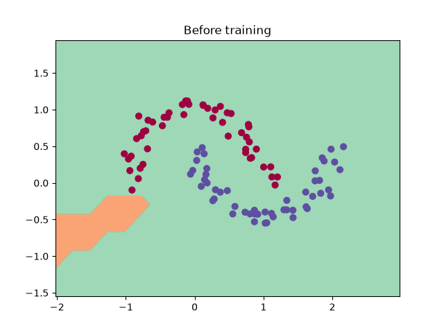
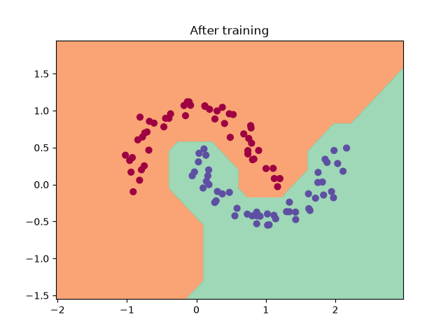
I trained an MLP(2, [16, 16, 1]) on the classic two-interleaved-crescents make_moons dataset:
step 0:  loss 1.4665, accuracy 26.0%
step 20: loss 0.0984, accuracy 96.0%
step 60: loss 0.0182, accuracy 100.0%
Scaling up: one Value per number doesn't scale
The scalar engine builds a new graph for every training step, one node per number, so a 100-example batch through a [2,16,16,1] network allocates thousands of Python objects. Tensor is the same structure, except data is a NumPy array instead of a float. One node represents a whole matrix. A single matmul replaces hundreds of scalar ops.
Most of Tensor is a direct generalization of Value. Two parts weren't: broadcasting and softmax.
Broadcasting has to be undone on the way back
NumPy broadcasts silently: adding a (4,) vector to a (3,4) matrix just works. Broadcasting creates multiple consumers of the same value, so the backward pass must sum the gradient across the broadcast dimensions to undo it.
Concretely, if b has shape (4,) broadcast up to (3,4) inside a + b, then for each j:
One generic helper handles it rather than special-casing every op:
def _unbroadcast(grad, shape):
    while grad.ndim > len(shape):          # broadcast added new leading axes
        grad = grad.sum(axis=0)
    for i, dim in enumerate(shape):        # broadcast stretched a size-1 axis
        if dim == 1 and grad.shape[i] != 1:
            grad = grad.sum(axis=i, keepdims=True)
    return grad
Every binary op runs its gradient through this before accumulating.
For matmul, , the gradients are:
np.swapaxes(-1, -2) instead of a plain transpose handles batched matmuls by only swapping the last two axes. A batched input against an unbatched weight matrix goes through the same _unbroadcast helper.
Softmax: the one op where the "local gradient" isn't a number
Every other op has a scalar or elementwise local gradient. Softmax doesn't, because every output depends on every input. Its local gradient is a full Jacobian:
Given an upstream gradient , the chain rule sums over :
That collapses into a single elementwise formula:
dot = np.sum(out.grad * out.data, axis=axis, keepdims=True)   # Σᵢ gᵢsᵢ
self.grad += out.data * (out.grad - dot)                       # s · (g − Σgs)
The full Jacobian never has to be formed explicitly: the sum over i reduces to a single dot product between out.grad and out.data, after which the remaining computation is elementwise. The forward pass also subtracts before exponentiating. This is exact, not an approximation: for any constant . It keeps exp() from overflowing on large inputs.
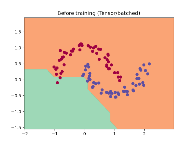
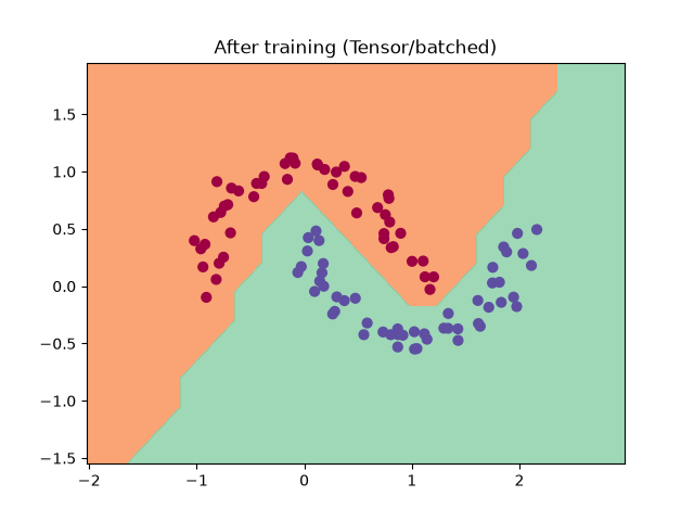
The Tensor implementation produces the same decision boundary while replacing thousands of scalar graph nodes with vectorized NumPy operations.
What I learned
- Reverse-mode autodiff is conceptually simple; most implementation complexity comes from bookkeeping around graph traversal and gradient accumulation.
- Generalizing from scalars to tensors introduces new concerns, particularly broadcasting semantics and batched linear algebra, rather than changing the underlying differentiation algorithm.
- Building higher-level operations from verified primitives substantially reduces the amount of backward logic that must be implemented and tested.
What's next
The next step is implementing a character-level transformer using this engine. Remaining work includes embedding lookup with scatter-add gradients, layer normalization, and a logarithm primitive for cross-entropy loss. Each requires implementing additional local gradient rules while reusing the existing reverse-mode engine.